Single record animal model in ASReml

A single record animal model is the simplest, and probably most important, linear mixed model (LMM) used in animal breeding. This model is called animal model (or individual model) because we estimate a breeding value for each animal defined in the pedigree. The term single record refers to the fact that animals have only one phenotypic observation available (in contrast with repeated measures, where we have multiple records for each individual).

Breeding values are random effects estimated as part of fitting the LMM, and these correspond to the genetic worth of an individual. In the case of progenitors, this is obtained as the mean deviation of the offspring of the given parent against the population mean. Breeding values are used to select individuals to constitute the next generation. 

In this blog we will present an analysis from a swine breeding program where the model has several fixed effects and a single additive genetic effect. The base model is:

where  

is the phenotypic observation of animal
is the overall mean
is a fixed effect such as contemporary group
is the random additive genetic value of animal
is the random residual terms

The fixed effects  in this case correspond to contemporary groups, but these effects can be any general nuisance factor or continuous variables of interest to control for, such as herds, year, season (also constructed as a single factor often called hys), sex, or some continuous variables to be used as covariates such as initial size or weight.

In the above model, we have distributional assumptions associated with the random effects, specifically, a ~ MVN(0, A) and e ~ MVN(0, I). Here, the vector of breeding values a has a mean of zero and they have a variance-covariance matrix A that corresponds to the numerator relationship matrix, and  is the variance of additive effects (i.e.,  = VA). In addition, the vector of residuals has a mean of zero and they have an identity variance-covariance matrix (i.e., independent effects) with  being the error or residual variance.     

The above model is fitted with ASReml v4.1 using residual maximum likelihood (REML) to estimate variance components: fixed and random effects (i.e., BLUEs and BLUPs) are obtained by solving the set of mixed model equations.

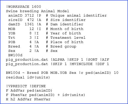
In ASReml we write a text file (with the extension ‘.as’) with all the specifications of the dataset to be used, together with the details of the model to be fitted. The full code is presented below:

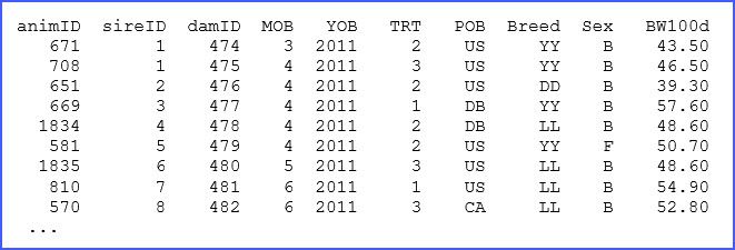
There are many elements in the above code, only a few of which we will discuss here, but more information can be found in the manual. The structure of the dataset ‘pig_production.dat’ and a brief description is presented in lines 2 to 11, and for reference we present a few of the lines of this dataset below:

Some of the descriptions of these variables in the ‘.as’ file are critical. For example, !P is used to indicate that the factor animID is associated with a pedigree file that will be the first file to read. The use of !I and !A is used for specification of factors coded as integers or alphanumeric, respectively. When no qualifier is present the data column will be considered as a continuous real variable, such as with BW100d.

In this example, the use of !P requires the reading of a pedigree file, which is critical for fitting an animal model, and in our example this file is the same as the data file. This is possible because the first three columns of the dataset correspond to the ones required for the pedigree: Animal, Sire and Dam. Additional qualifiers are used for reading these files, such as !SKIP and !ALPHA.

In addition, there are two important qualifiers associated with the analysis. These are: !MVINCLUDE, which is required to keep the missing records associated with some of the factors, and the !DDF 1 qualifier that requests the calculation of an ANOVA table associated with our model using approximated degrees of freedom.

Finally, we find the model specification lines:

The first term BW100d is the response variable. Then the following four terms Breed, POB, MOB.YOBand SEXare fixed effect factors. Here MOB.YOB corresponds to a combined factor of all combinations of MOB and YOB (recall these are month and year of birth, respectively). Then the use of !r precedes the definition of random effects; here the only term used is ped(animID), which is the animal effect associated with pedigree. The use of ped() is optional here, as the model term animID was previously read with the qualifier !P before, but this is good practice. Also note that we added a value 10 after this random effect; this is to assist the software with an initial guess of the additive variance component.

The second line is required to define complex variance structures for residual terms. However, in this case we have a simple structure based on independent errors with a single variance (i.e., idv) and this is defined for all units that correspond to each observation. Other structures for random effects and the residual term are possible, and further details can be found in the manual.

After fitting the model, a series of output files are produced with the same basename file, but with different filename extensions. The most important outputs for the animal model of above are: ‘.asr’, ‘.sln’, and ‘.pvc’.

The ‘.asr’ file contains a summary of data, the iteration sequence, estimates of the variance parameters, and the analysis of variance table together with estimates of the fixed effects, among many other things, and also messages. In our dataset, the additive genetic and residual variances for BW200d were estimated to be 11.14 and 79.49 kg, respectively. Fixed effect tests for this trait show highly significant differences (p < 0.01) for most factors, as shown below in an excerpt of this file.

Note that there is additional output in the file ‘.asr’ and probably more that you normally will need. Refer to the manual for additional details and definitions.

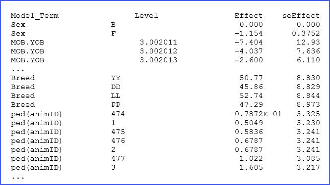
The file ‘.sln’ has the solutions (BLUEs and BLUPs) from our analysis. A few lines of this output are presented below:

There are columns to identify the factor and its levels followed by the estimated effect and associated standard error. For example, for animal 477, we note that its BLUE effect (in this case breeding value) is 1.022 kg above the mean. The complete list should help to select the best individuals for this swine breeding study.

There was one additional element from the ‘.as’ file that we did not describe, and this corresponds to the command !VPREDICT that is used to request the additional estimation of the narrow-sense heritability; this will be reported in the ‘.pvc’ file. The lines used corresponded to:

Here we are requesting ASReml to generate a ‘.pin’ file with our variance prediction function request. In this case, we will first take the variance associated with ped(animID) and call it AddVar, then we sum the variance for animID and the residual variance (identified as idv(units)). Finally, we take these two elements and divide them. Hence, we just defined the expression: = /(). In the file ‘.pvc’ you will notice the following output:

The heritability for BW100d is 0.123 ± 0.034. Note that, as indicated, standard errors are approximated as this calculation uses the Delta method.

There is another relevant output found in the file ‘.aif’ that reports calculations of each individual’s inbreeding coefficient. This is relevant for selection and control of inbreeding in a program. ASReml produced this additional output because we used the !AIF qualifier, but we have not presented the output in this blog.

ASReml has many other options and it can handle large databases and fit many complex linear models. Here we only presented a few of its capabilities, but if you want to learn more about ASReml check the online resources here. You can find more details of this product at https://www.vsni.co.uk/software/asreml.